Backpropagation Algorithm
Backpropagation is the foundational algorithm for training multilayer neural networks. It efficiently computes gradients of the loss function with respect to all weights, enabling gradient-descent learning.
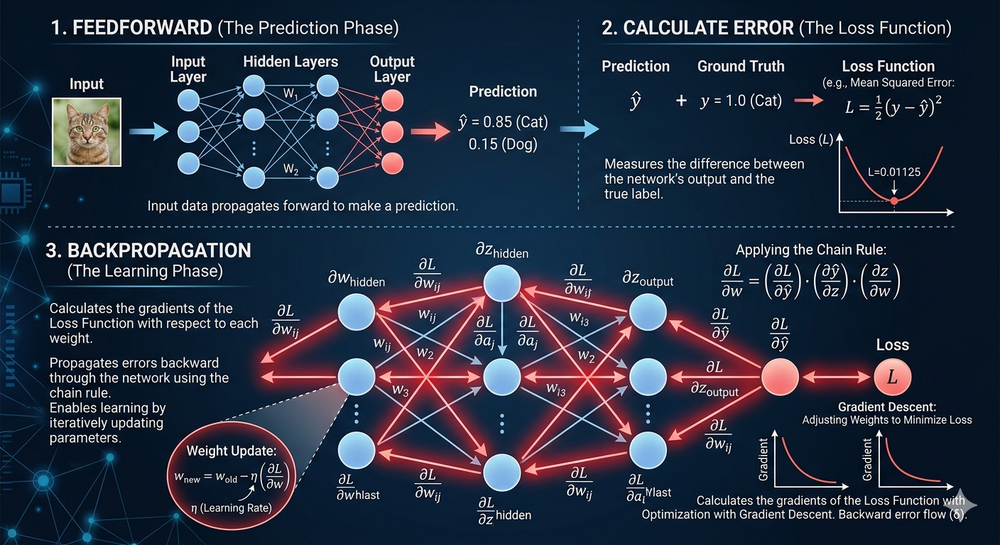 The complete backpropagation process: (1) Feedforward prediction, (2) Calculate loss/error, (3) Backpropagate errors (red arrows) using chain rule to compute gradients, then update weights via gradient descent.
Problem Statement
Given: - Training examples with input x and target output y - Neural network with weights w - Loss function: Loss(w) = |y - h_w(x)|²
Find: - Weights w that minimize total loss - Gradient: ∂Loss/∂w for each weight w
Key Insight: Chain Rule
The loss depends on weights through a chain of compositions:
Loss ← output layer ← hidden layer ← ... ← input layer ← weights
Backpropagation uses the chain rule to efficiently compute gradients: - Forward pass: Compute all activations a_i - Backward pass: Compute error terms Δ and propagate backward - Weight updates: Change weights proportionally to ∂Loss/∂w
Algorithm Steps
Step 1: Forward Propagation
For each layer ℓ from input to output:
inⱼ = Σᵢ wᵢⱼ aᵢ    (weighted sum of inputs)
aⱼ = g(inⱼ)       (apply activation function)
Result: Compute all activations a for all nodes.
Step 2: Compute Output Error
At output layer k:
Δₖ = (yₖ - aₖ) × g'(inₖ)
Where: - (yₖ - aₖ): Raw error at output - g'(inₖ): Derivative of activation (how sensitive is output to change in input)
Step 3: Backpropagate Errors
For each hidden layer ℓ from output to input:
Δⱼ = g'(inⱼ) × Σₖ wⱼₖ Δₖ
Intuition: - Hidden unit j is responsible for errors Δₖ in all units k it connects to - Responsibility weighted by connection strength wⱼₖ - Scaled by activation derivative g'(inⱼ)
Step 4: Update Weights
For all weights w_ij:
w_ij ← w_ij + α × a_i × Δ_j
Where: - α: Learning rate (how much to adjust) - a_i: Activation of upstream unit (input signal) - Δ_j: Error responsibility of downstream unit
Interpretation: - Increase weight if both a_i and Δ_j positive (both want same direction) - Decrease if opposite signs - Learning proportional to strength of signals
Mathematical Derivation
For output layer weight w_jk:
∂Loss/∂w_jk = -2(y_k - a_k) × g'(in_k) × a_j
            = -a_j × Δ_k
For hidden layer weight w_ij (chain rule applied recursively):
∂Loss/∂w_ij = -a_i × g'(in_j) × Σₖ w_jk × Δ_k
            = -a_i × Δ_j
Key observation: Same update rule applies at all layers!
Computational Efficiency
Why not compute gradients separately for each weight? - Direct approach: O(w²) computation (recalculate paths) - Backpropagation: O(w) computation (reuse intermediate results) - Exponential speedup: 10-layer network: millions of weights, O(w) instead of O(w²)
Key insight: Reverse-mode automatic differentiation - Forward pass: Store all activations (O(n) memory) - Backward pass: Reuse stored values to compute gradients
Important Details
Multi-Output Networks
For networks with multiple outputs:
∂Loss/∂w = Σₖ ∂Loss_k/∂w
Decompose m-output problem into m learning problems: - Compute Δ_k for each output independently - Sum gradient contributions before weight update
Weight Initialization
Initialize weights: - Small random values (e.g., uniform [-0.01, 0.01]) - NOT zero: All units would learn same thing - NOT large: Can cause saturation (near bounds of sigmoid)
Activation Function Derivative
Sigmoid: g'(x) = g(x) × (1 - g(x)) - Can derive g' from output: g'(x) = a × (1 - a) where a = g(x) - Efficient: Compute once during forward pass
ReLU: g'(x) = 1 if x > 0, else 0 - Simple, efficient, avoids vanishing gradient - (Modern networks use ReLU instead of sigmoid)
Learning Rate α
- Too large: Oscillate, diverge
- Too small: Very slow convergence
- Adaptive rates (momentum, Adam): Adjust α during training
Stopping Criteria
Training-based: - Fixed iterations (e.g., 1000 epochs) - Training loss below threshold
Validation-based (preferred): - Monitor error on separate validation set - Stop when validation error increases (overfitting sign) - Return best weights seen during training
Vanishing Gradient Problem
In deep networks with sigmoid:
Δ ∝ g'(x) where g'(x) ≤ 0.25
After many layers: Δ_1 ∝ g'×g'×...×g' ≈ (0.25)^L → near zero
Solutions: - Use ReLU: g'(x) = 1 (not ≤ 0.25) - Batch normalization: Normalize layer inputs - Careful initialization: Xavier/He initialization - Skip connections: Allow gradients to bypass layers
Related Concepts
- Neural-Networks — Architecture and theory
- Gradient-Descent — General optimization framework
- Machine-Learning — Learning paradigm
- Deep-Learning — Multi-layer networks, modern variants
- Chain-Rule — Mathematical foundation
References
Russell & Norvig (2010): Chapter 18.7 - Artificial Neural Networks & Backpropagation