Artificial Neural Networks
Neural Networks are computational models inspired by biological neural systems. They learn by adjusting weights connecting artificial neurons, enabling them to approximate complex nonlinear functions.
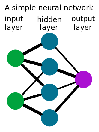 A simple neural network with input layer, hidden layer, and output layer. Connections represent weighted parameters learned during training.
Architecture
Basic Unit: Perceptron
- Input: Vector of real-valued inputs
- Weights: w₀ (bias), w₁, w₂, ... (connection strengths)
- Activation: a = g(w₀ + Σᵢ wᵢ aᵢ)
- g: Activation function (sigmoid, ReLU, tanh)
Network Structure
Layers: - Input layer: Raw features - Hidden layer(s): Learned representations - Output layer: Final predictions
Connectivity: - Fully connected: Every neuron connects to next layer - Sparse: Selective connections - With/without skip connections (modern architectures)
Depth: - Single hidden layer: Universal approximators (with enough units) - Multiple layers: Can represent functions more efficiently - Deep networks: 3+ hidden layers (deep learning)
Activation Functions
Sigmoid: g(x) = 1 / (1 + e⁻ˣ) - Smooth, differentiable, outputs [0,1] - Historically important - Prone to vanishing gradients in deep networks
Tanh: g(x) = (e²ˣ - 1) / (e²ˣ + 1) - Outputs [-1, 1] - Steeper gradient than sigmoid - Better for hidden layers
ReLU (Rectified Linear Unit): g(x) = max(0, x) - Simple, fast, avoids vanishing gradient problem - Standard in modern deep learning - Dead neuron problem with naive training
Softmax: For multi-class output - Outputs probability distribution - Standard for classification output layer
Universal Approximation
Theorem: A network with one sufficiently large hidden layer can approximate any continuous function on compact domain with arbitrary accuracy.
Caveat: Number of hidden units grows exponentially with input dimension in worst case
Practical implication: - Single layer sufficient theoretically - Multiple layers often more sample-efficient - Two layers can represent discontinuous functions
Nonlinear Regression
Neural networks perform nonlinear regression: - Compose nonlinear soft thresholds (hidden units) - Combinations create complex bump/ridge patterns - Sufficient units create arbitrary nonlinear surface
Example: Combining two opposite-facing sigmoid functions → ridge. Two perpendicular ridges → bump pattern. Scale: more units → more features.
Learning: Backpropagation
Core Idea
Learn weights by minimizing loss function via gradient descent: - Forward pass: Compute outputs - Backward pass: Propagate errors (Δ values) to adjust weights - Repeat until convergence
Forward Propagation
For each layer ℓ = 2 to L:
inⱼ = Σᵢ wᵢⱼ aᵢ  (weighted input)
aⱼ = g(inⱼ)      (activation)
Error Backpropagation
Output layer:
Δₖ = (yₖ - aₖ) × g'(inₖ)
Hidden layers (backward from output):
Δⱼ = g'(inⱼ) × Σₖ wⱼₖ Δₖ
Weight Updates
wᵢⱼ ← wᵢⱼ + α × aᵢ × Δⱼ
Algorithm (BACK-PROP-LEARNING)
- Initialize weights randomly (small values)
- For each training example: a. Forward pass: compute outputs b. Backward pass: compute Δ values layer by layer c. Update weights: wᵢⱼ ← wᵢⱼ + α × aᵢ × Δⱼ
- Repeat until stopping criterion (error threshold, iterations, etc.)
Key Properties
Advantages
- Universal approximators (with hidden layers)
- Learn complex nonlinear functions
- Parallel computation (fast with GPU)
- Handle vector inputs naturally
- Can learn hierarchical representations (deep networks)
Challenges
- Local minima: Gradient descent finds local, not global optima
- Vanishing gradient: Gradients shrink in deep networks (sigmoid)
- Overfitting: Large networks on small datasets
- Black box: Hard to interpret learned weights
- Hyperparameter sensitivity: Learning rate, layer sizes, etc.
Improvements (Modern)
- Batch normalization: Stabilize training
- Dropout: Reduce overfitting
- ReLU activation: Avoid vanishing gradients
- Momentum/Adam optimizers: Better convergence
- Early stopping: Stop when validation error increases
Training
Loss Functions
- L₂ loss (regression): Loss = Σₖ (yₖ - aₖ)²
- Cross-entropy (classification): -Σₖ yₖ log(aₖ)
- L1 loss (robust): Σₖ |yₖ - aₖ|
Stopping Criteria
- Fixed number of iterations
- Validation error stops improving (early stopping)
- Training error reaches threshold
- Manual inspection of learning curves
Cross-Validation
Try different network structures (# layers, units): - Simple structures: Risk underfitting - Complex structures: Risk overfitting - Use validation set to find sweet spot
Related Concepts
- Backpropagation — Detailed learning algorithm
- Gradient-Descent — General optimization approach
- Machine-Learning — Broader learning framework
- Deep-Learning — Multiple layers, modern architectures
- Convolutional-Networks — Specialized for images
- Recurrent-Networks — Specialized for sequences
References
Russell & Norvig (2010): Chapter 18 - Artificial Neural Networks