Logistic Regression¶

Logistic regression is a supervised learning algorithm for binary classification. Despite its name, it's a classification method (not regression). It models the probability that an input belongs to a specific class using a logistic (sigmoid) function.

Core Concept¶

Logistic regression uses the logistic function to map continuous outputs to probabilities:

P(y=1|x) = σ(w₀ + w₁x₁ + w₂x₂ + ... + wₙxₙ)

Where σ is the sigmoid function:

σ(z) = 1 / (1 + e^(-z))

This produces output between 0 and 1, interpretable as: - P(y=1|x) = Probability input belongs to class 1 - P(y=0|x) = 1 - P(y=1|x)

The Sigmoid Function¶

The sigmoid (logistic) function:

σ(z) = 1 / (1 + e^(-z))

Properties: - Output always between 0 and 1 - Smooth, differentiable curve - S-shaped: flat at extremes, steep in middle - Threshold at z=0: σ(0) = 0.5

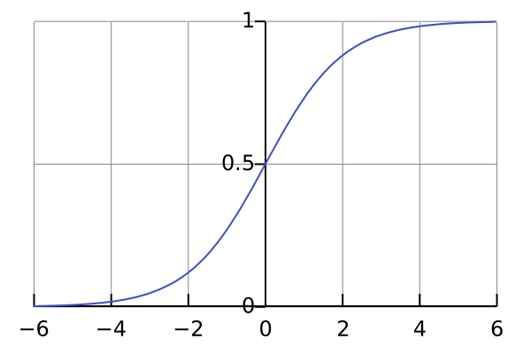Logistic Sigmoid Curve The sigmoid function maps any input to a probability between 0 and 1. The curve is S-shaped with inflection point at z=0, σ(0)=0.5.

Decision boundary: Typically classify as: - Class 1 if P(y=1|x) ≥ 0.5 (i.e., σ(z) ≥ 0.5) - Class 0 otherwise

Learning Algorithm¶

Objective¶

Minimize cross-entropy loss (log loss):

Loss = -Σᵢ [yᵢ log(ŷᵢ) + (1-yᵢ) log(1-ŷᵢ)]

Where: - yᵢ = actual class (0 or 1) - ŷᵢ = predicted probability P(y=1|x)

Intuition: - If y=1, loss decreases as ŷ increases (want high probability) - If y=0, loss decreases as ŷ decreases (want low probability)

Optimization¶

Use [[gradient-descent|gradient descent]] to iteratively update weights:

w ← w - α∇Loss

Gradient of cross-entropy loss:

∂Loss/∂w = Σᵢ (ŷᵢ - yᵢ) xᵢ

Note: Unlike linear regression, logistic regression has no closed-form solution.

Binary Classification¶

Logistic regression naturally handles binary (2-class) problems:

Class 0: Negative class (absence of condition)
Class 1: Positive class (presence of condition)

Examples: - Email: Spam (1) vs. Not spam (0) - Medical: Disease present (1) vs. Absent (0) - Credit: Default (1) vs. No default (0)

Multi-class Extension: One-vs-Rest¶

For multi-class problems (K > 2 classes), train K binary classifiers:

Train classifier 1: Class 1 vs. Rest
Train classifier 2: Class 2 vs. Rest
... (for each class)

Prediction: Pick class with highest probability

Comparison to [[linear-regression]]¶

Aspect	Linear Regression	Logistic Regression
Output	Continuous (any real value)	Probability (0-1)
Task	Regression	Classification
Loss function	Mean squared error	Cross-entropy
Boundary	Continuous line/plane	Decision boundary
Example	Predict house price	Predict spam/not-spam

Advantages & Limitations¶

✅ Advantages¶

Probabilistic output: Returns probabilities, not just class labels
Interpretable: Weights show feature importance/direction
Efficient: Fast training, works on large datasets
Robust: Handles multi-class via one-vs-rest
Well-studied: Extensive statistical theory

❌ Limitations¶

Linear boundary: Can't model complex nonlinear decision boundaries
Assumes independence: Features should be somewhat independent
Sensitive to outliers: Extreme examples can affect probabilities
Requires scaling: Features should be normalized for stable training
Binary focus: Multi-class requires workarounds

Decision Boundary¶

Logistic regression creates a linear decision boundary:

P(y=1|x) = 0.5  when  w₀ + w₁x₁ + w₂x₂ + ... = 0

This is a hyperplane (line in 2D, plane in 3D, etc.)

Limitation: If classes require nonlinear separation, logistic regression will underfit.

Solution: Use [[neural-networks|neural networks]] or [[support-vector-machines|kernel methods]] for nonlinear boundaries.

Regularization¶

To prevent overfitting, add regularization term:

Loss = -Σᵢ [yᵢ log(ŷᵢ) + (1-yᵢ) log(1-ŷᵢ)] + λ||w||²

Effect: - Penalizes large weights - Encourages simpler, more generalizable models - λ controls regularization strength

Practical Implementation¶

Training: 1. Initialize weights (typically to 0) 2. For each iteration: - Compute predictions ŷ = σ(Xw) - Compute loss - Update weights via gradient descent - Check convergence

Prediction: 1. Compute z = w₀ + w₁x₁ + ... 2. Compute P(y=1|x) = σ(z) 3. If P ≥ 0.5: predict class 1, else class 0

Common Use Cases¶

Email filtering: Spam detection
Medical diagnosis: Disease detection from symptoms
Credit scoring: Loan default prediction
Customer churn: Predicting customer attrition
Ad targeting: Click-through rate prediction
Sentiment analysis: Positive vs. negative text classification

[[Linear-Regression]] — Foundation model
[[Machine-Learning]] — Supervised learning paradigm
[[Neural-Networks]] — Nonlinear extension via hidden layers
[[Support-Vector-Machines]] — Kernel-based classification
[[Gradient-Descent]] — Optimization method
[[Regularization]] — Preventing overfitting

References¶

Wikipedia: Logistic Regression
Russell & Norvig (2010): Chapter 18 - Machine Learning